Multivariate Normal distribution and Cholesky decomposition in Stan

Figure 1: Simulated data in a Multivariate Normal distribution

This post provides an example of simulating data in a Multivariate Normal distribution with given parameters, and estimating the parameters based on the simulated data via Cholesky decomposition in stan. Multivariate Normal distribution is a commonly used distribution in various regression models and machine learning tasks. It generalizes the Normal distribution into multidimensional space. Its PDF can be expressed as:

where mu is a vector of k elements for the location parameters and Sigma is the Variance-Covariance matrix. The |Sigma| calculates the absolute determinant of Sigma in the equation above.

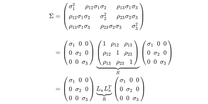
Cholesky decomposition is used to decompose a positive-definite matrix into the product of a lower triangular matrix and its transpose. In our case, we will decompose the correlation matrix (R) into the product of two triangular matrices (L*L’). Note: even though we can directly perform Cholesky decomposition on the Variance-Covariance matrix (Sigma), it is not recommended, since we may fail to estimate the standard deviations (sigma) of each variable.

Matrix representation of Cholesky decomposition

1. Data simulation

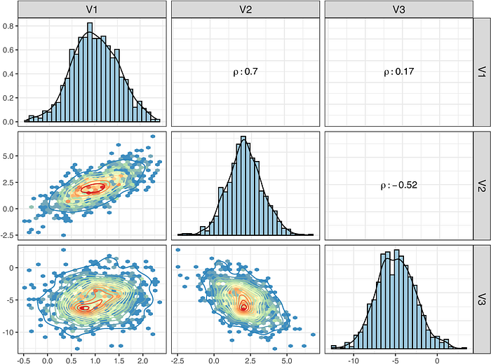
The variance-covariance matrix (Sigma) for data simulation and its analytical solution via Cholesky decomposition are provided below. For example, the standard deviation for the first variable sd_1 is 0.5, and the correlation coefficient (rho) between first and second variables is 0.7 (see Figure 1 for more intuitive illustration).

Decomposing an example correlation matrix (R) via Cholesky factorization

To generate the data, we are using the mvrnorm function from the package MASS by specifying a vector of means (mu) and variance-covariance matrix (Sigma).

mu = c(1, 2, -5) # means
R = matrix(c(1, 0.7, 0.2, # correlation matrix (R)
             0.7, 1, -0.5,
             0.2, -0.5, 1), 3)
sigmas = c(0.5, 1.2, 2.3) # sd1=0.5, sd2=1.2, sd3=2.3
Sigma = diag(sigmas) %*% R %*% diag(sigmas) # VCV matrix
data = mvrnorm(1000, mu = mu, Sigma = Sigma) #…